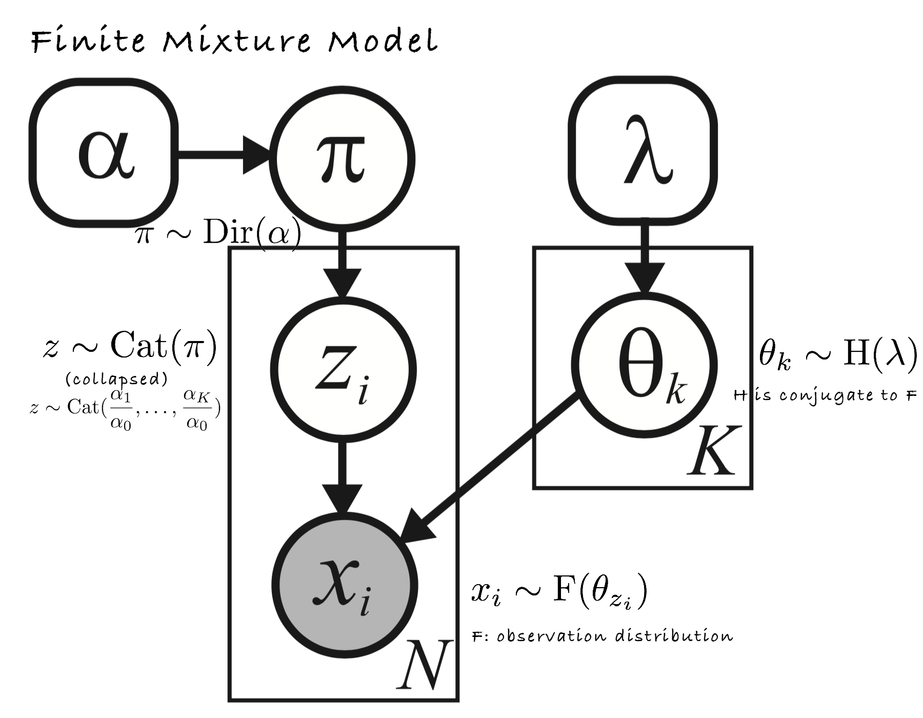
Start from finite mixture model...
Traditional representation:

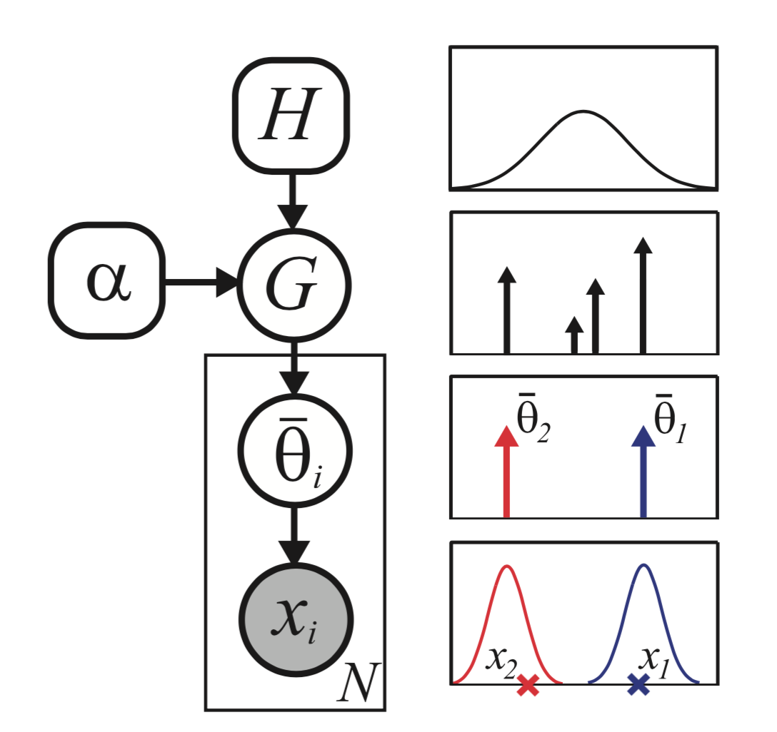
Another representation (in which H and F are both Gaussian):

where parameters are sample from G, a discrete measure of
and
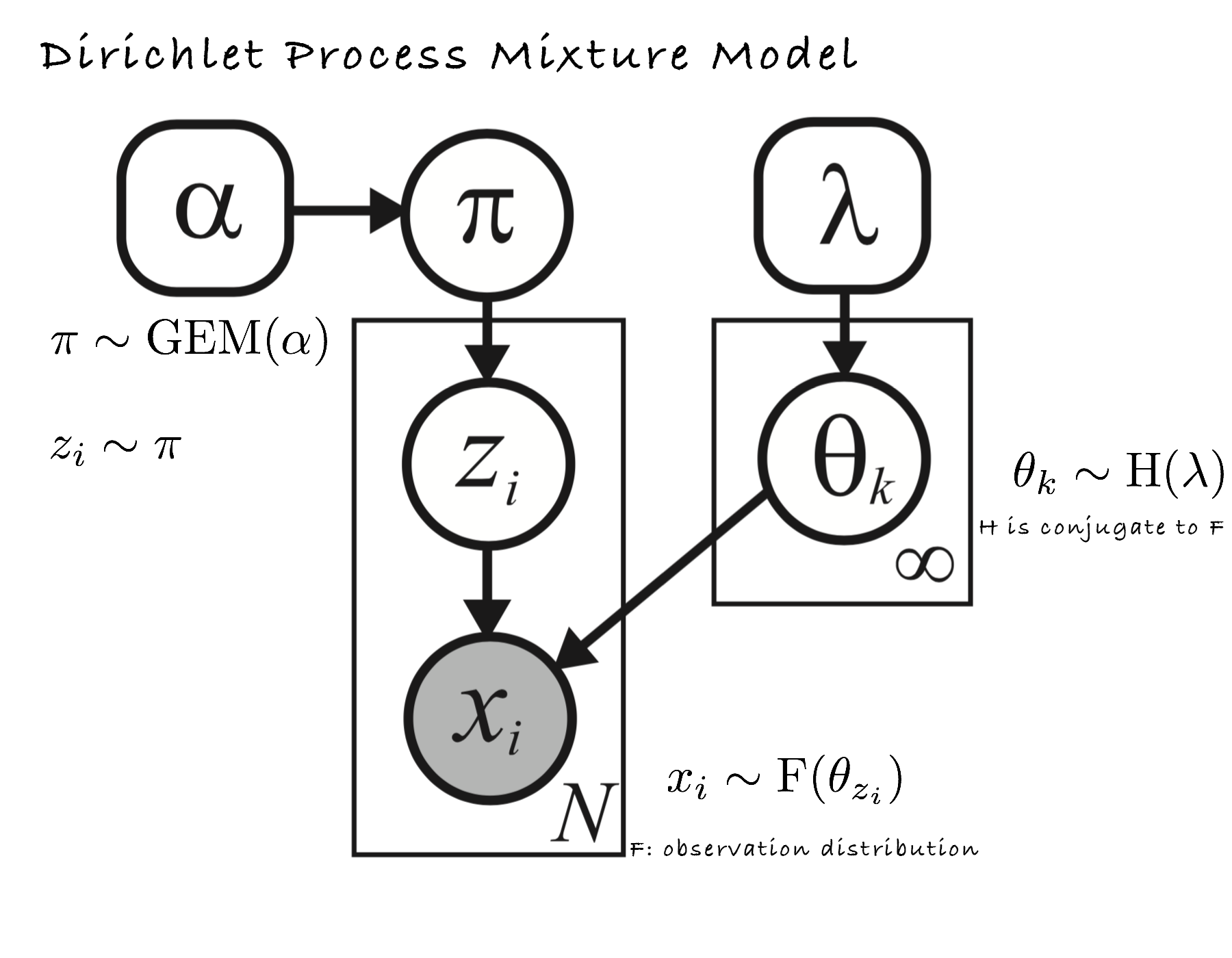
DPMM

Another representation:

Where
One can show that the GEM process will terminate with probability 1, which means samples from a DP are discrete with probability 1. As
model fitting (Gibbs sampling)
where
Example: DPMM algorithm for clustering:
Random initial assignment to clusters
loop
  unassign an observation
  choose new cluster for that observation
until convergence
Gibbs sampling for choosing cluster:
on the assumption that base distribution G is normal distribution with zero mean and unit variance.
Reference
"Machine Learning" Lecture 17: http://www.umiacs.umd.edu/~jbg/teaching/CSCI_5622/
Book: Machine Learning - A Probabilistic Perspective(Chapter 25)